Félix Abecassis

In this article we will present a simple code finding an optimal solution to the graph coloring problem using Integer Linear Programming (ILP). We used the GNU Linear Programming Kit (glpk) to solve the ILP problem.

Background

As a project assignment for school we recently had to implement an optimized MPI program given a undirected graph where the edges represent the communications that should take place between MPI processes. For instance this program could be used for a distributed algorithm working on a mesh where each MPI process work on a share of the whole mesh, the edges represent the exchange of boundaries conditions for each iteration.
For a given process, the order of communications with all the neighbours is highly correlated with the performance of the whole program. If all processes start by sending data to the same process, the network bandwidth to this process will be a bottleneck. Therefore it is important to find a good order for communications. Ideally, at each step one process should be involved in only one communication.

By coloring the edges of the graph (all adjacent edges must have different colors), we can find a good scheduling order for MPI communications. Edge coloring can be solved directly, but we have chosen to use the line graph (also called edge-to-vertex dual) instead of the original graph. Therefore we just have to color the vertices of the line graph instead of implementing an edge coloring algorithm.

Goal

Initially we implemented a greedy coloring algorithm using the Welsh-Powell heuristic. This algorithm is fast and generally yields fairly good results, but I was interested in getting the optimal solution. Remembering the course I had on linear programming and the research papers I read on register allocation, I decided to use integer linear programming to solve this problem. The proposed implementation is by no means optimized, my goal was to implement a simple but optimal solution using a linear programming library. The final code is approximately 100 lines of code and I think it can be an interesting example for developers that want to start using GLPK.

Input

We need an input format to describe our graph. We used a very simple file format: each line is a vertex, the first number on each line is the identifier of the vertex and the remaining numbers are the neighbours of this vertex. For instance, Wikipedia provides the following example for graph coloring:

Labelling the vertices from 0 to 5, we obtain the following file:

0 1 2 4 5
1 0 2 3 5
2 0 1 3 4
3 1 2 4 5
4 0 2 3 5
5 0 1 3 4

You will find other graph examples here:
- A bipartite graph (2-colorable, a greedy coloring algorithm can find colors).
- The smallest graph that fails the DSATUR heuristic (3-colorable, DSATUR finds 4 colors).
- The Grötzsch graph (4-colorable).
- Graph , i.e. complete graph with 5 vertices (5-colorable).
- The Petersen graph (3-colorable).

Linear Programming formulation

We implemented the LP formulation given by Mehrotra and Trick (the "VC" formulation).

The number of colors used by our solution is stored in an integer variable .
Given an upper bound on the number of colors needed, we use binary variables: if vertex is assigned color .

The objective function is simply:

Now we need to define the set of constraints for the graph coloring problem.
With the first constraint we state that each vertex must be assigned exactly one color:

The second constraint is a little tricky, we ensure that we use at most colors by stating that all columns using colors indices greater than are not used, i.e.:

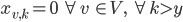
However, we can't use this formula in linear programming so we have to rewrite it:

Last but not least, we still need to ensure that adjacent vertices are assigned different colors:

GLPK Implementation

This article is not an introduction to GLPK but the library is simple to use if you have basic knowledge in linear programming, therefore I will not explain the GLPK functions used.

Our function will take as input the graph as a vector of vectors, this the same representation than the input file but with the current vertex index removed from each line.

void color_graph(const std::vector<std::vector<int> >& g)
{

We start by creating a problem object using GLPK and we set up the objective function:

  glp_prob* prob = glp_create_prob();
  glp_set_obj_dir(prob, GLP_MIN); // minimize

Before creating variables, we need an upper bound on the number of colors needed for our graph. Every graph can be colored with one more color than the maximum vertex degree, this will be our upper bound:

  int num_vertices = g.size();
  int max_colors = 0;
  for (int i = 0; i < num_vertices; ++i)
    max_colors = std::max(int(g[i].size()) + 1, max_colors);

As we have an upper bound for integer variable , we can create it and add it to the objective function:

  int y = glp_add_cols(prob, 1);
  glp_set_col_bnds(prob, y, GLP_DB, 1, max_colors); // DB = Double Bound
  glp_set_obj_coef(prob, y, 1.);
  glp_set_col_kind(prob, y, GLP_IV); // IV = Integer Variable

We now need to allocate and set the type of the binary variables . The indices are stored in a vector of vectors because we will need the indices while creating the constraints:

  std::vector<std::vector<int> > x(num_vertices, std::vector<int>(max_colors));
  for (int v = 0; v < num_vertices; ++v) 
    for (int k = 0; k < max_colors; ++k)
    {
      x[v][k] = glp_add_cols(prob, 1);
      glp_set_col_kind(prob, x[v][k], GLP_BV); // BV = Binary Variable
    }

To set up the constraints we must build the sparse matrix of coefficients by creating triplets .
These triplets are scattered in 3 different vectors. We must insert one element at the beginning because GLPK starts at index 1 after loading the matrix:

  std::vector<int> rows(1, 0);
  std::vector<int> cols(1, 0);
  std::vector<double> coeffs(1, 0.);

We now fill the three vectors by adding all the constraints (i.e. the rows) to the matrix, the first constraint:

  // One vertex must have exactly one color:
  // for each vertex v, sum(x(v, k)) == 1
  for (int v = 0; v < num_vertices; ++v)
  {
    int row_idx = glp_add_rows(prob, 1);
    glp_set_row_bnds(prob, row_idx, GLP_FX, 1, 1); // FX: FiXed bound
    for (int k = 0; k < max_colors; ++k)
    {
      rows.push_back(row_idx); 
      coeffs.push_back(1);
      cols.push_back(x[v][k]);
    }
  }

The second constraint:

  // We ensure we use y colors max:
  // for each vertex v and for each color c,                
  //    y >= (k + 1) * x(v, k)
  for (int v = 0; v < num_vertices; ++v)                    
  {
    for (int k = 0; k < max_colors; ++k)
    {
      int row_idx = glp_add_rows(prob, 1);
      glp_set_row_bnds(prob, row_idx, GLP_LO, 0, -1); // LO = LOwer bound
 
      rows.push_back(row_idx);
      coeffs.push_back(1);
      cols.push_back(y);                      
 
      rows.push_back(row_idx);
      coeffs.push_back(- k - 1);
      cols.push_back(x[v][k]);
    }
  }

And now the last set of constraints, this is a bit longer because we iterate on all edges. The graph is undirected but edges are duplicated in our file format, so we must ensure we do not add constraints twice:

  // Adjacent vertices cannot have the same color:        
  // for each edge (src, dst) and for each color k,                         
  //    x(src, k) + x(dst, k) <= 1                                          
  for (int src = 0; src < num_vertices; ++src)
  {
    const std::vector<int>& succs = g[src];
    for (int s = 0; s < succs.size(); ++s)
    {
      int dst = succs[s];
      // Ensure we don't add both (u, v) and (v, u)                                    
      if (src > dst)
      {
        for (int k = 0; k < max_colors; ++k)
        {
          int row_idx = glp_add_rows(prob, 1);
          glp_set_row_bnds(prob, row_idx, GLP_UP, -1, 1); // UP = UPper bound
 
          rows.push_back(row_idx);
          coeffs.push_back(1);
          cols.push_back(x[src][k]);
 
          rows.push_back(row_idx);
          coeffs.push_back(1);
          cols.push_back(x[dst][k]);
        }
      }
    }
  }

Everything is now set up! We must now load our sparse matrix into GLPK, ask GLPK to use the floating point solution as the initial solution (presolve) of our ILP problem and start the solver:

  glp_load_matrix(prob, rows.size() - 1, &rows[0], &cols[0], &coeffs[0]);
  glp_iocp parm;
  glp_init_iocp(&parm);
  parm.presolve = GLP_ON;
  glp_intopt(prob, &parm);

After the last call returns, we have a minimal coloring solution, we can now print the value of and :

  double solution = glp_mip_obj_val(prob);
  std::cout << "Colors: " << solution << std::endl;
  for (int i = 0; i < num_vertices; ++i)
  {
    std::cout << i << ": ";
    for (int j = 0; j < max_colors; ++j)
      std::cout << glp_mip_col_val(prob, x[i][j]) << " ";
    std::cout << std::endl;
  }
}

For instance on the provided bipartite graph we obtain:

Colors: 2
0: 0 1 0 0
1: 0 1 0 0
2: 0 1 0 0
3: 1 0 0 0
4: 1 0 0 0
5: 1 0 0 0

The last two columns are empty, this is because we started with an upper bound but we used only 2 colors.

Running

If you want to run the program, here a small main function to load a graph file and call our coloring algorithm:

int main(int argc, char** argv)
{
  std::vector<std::vector<int> > g;
  std::ifstream fs(argv[1]);                                                
  while (true)  
  {
    std::string line;
    std::getline(fs, line);
    if (fs.eof())
      break;
    std::istringstream iss(line);
    std::istream_iterator<int> begin(iss), eof;
    g.push_back(std::vector<int>(++begin, eof));
  }
  color_graph(g);
}

Thoughts

To end this article, here are some important points:
- If the initial bounds for is tight, solving will be faster. For the lower bound you can use 2 instead of 1 if your graph is not edgeless. To find a better upper bound you can use a greedy coloring algorithm before using ILP to find the optimal solution.
- If you want to solve the problem faster, use another formulation using column generation.
- If you use C++ you might want to implement your own wrapper above GLPK in order to manipulate variables and constraints easily.

Update

After reading my article, my teacher Anne-Laurence Putz kindly gave me another formulation which is simpler and generally more efficient.
We delete variable and use the following objective function instead: