Category Archives: OpenCV - Page 2

OpenCV - Morphological Skeleton

Skeleton

In many computer vision applications we often have to deal with huge amounts of data: processing can therefore be slow and requires a lot of memory.
In order to achieve faster processing and a smaller memory footprint, we sometimes use a more compact representation called a skeleton.
A skeleton must preserve the structure of the shape but all redundant pixels should be removed.
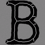
Here is a skeleton of the letter "B":

In this article we will present how to compute a morphological skeleton with the library OpenCV.
The skeleton obtained is far from perfect but it is a really simple method compared to other existing algorithms.

Pseudocode

As described on Wikipedia, a morphological skeleton can be computed using only the two basic morphological operations: dilate and erode.
In pseudo code, the algorithm works as follow:

img = ...;
while (not_empty(img))
{
    skel = skel | (img & !open(img));
    img = erosion(img);
}

At each iteration the image is eroded again and the skeleton is refined by computing the union of the current erosion less the opening of this erosion. An opening is simply an erosion followed by a dilation.

Implementation

It's really straightforward, first load the image to process in grayscale and transform it to a binary image using thresholding:

cv::Mat img = cv::imread("O.png", 0);
cv::threshold(img, img, 127, 255, cv::THRESH_BINARY);

We now need an image to store the skeleton and also a temporary image in order to store intermediate computations in the loop. The skeleton image is filled with black at the beginning.

cv::Mat skel(img.size(), CV_8UC1, cv::Scalar(0));
cv::Mat temp(img.size(), CV_8UC1);

We have to declare the structuring element we will use for our morphological operations, here we use a 3x3 cross-shaped structure element (i.e. we use 4-connexity).

cv::Mat element = cv::getStructuringElement(cv::MORPH_CROSS, cv::Size(3, 3));

And now the core of the algorithm, the main loop. We need a boolean variable in order to check if there is at least one pixel remaining. Operations are done in-place when possible.

bool done;
do
{
  cv::morphologyEx(img, temp, cv::MORPH_OPEN, element);
  cv::bitwise_not(temp, temp);
  cv::bitwise_and(img, temp, temp);
  cv::bitwise_or(skel, temp, skel);
  cv::erode(img, img, element);
 
  double max;
  cv::minMaxLoc(img, 0, &max);
  done = (max == 0);
} while (!done);

The use of the minMaxLoc function deserves an explanation. We want to check if there is still at least one pixel in the image, unfortunately I have not found a function for this task in OpenCV, therefore I just check if the maximum value is 0. minMaxLoc stores the minimum value in the second parameter (ignored if NULL pointer) and the maximum in the third parameter. A short-circuit OR function would be nice for this task.

The loop is over, we have our skeleton, let's display it!

cv::imshow("Skeleton", skel);
cv::waitKey(0);

Results

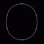
On a big "O":

On the word "OpenCV":

Optimization

As discussed with Arthur Kalverboer in the comments below, it is possible to optimize the computation in several ways.

First of all we can notice we perform the open operation and just after we perform an erosion on the same image, but an opening is just an erosion followed by a dilation, so we can perform the erosion and save it to a new image eroded, and at the end of the loop we copy eroded to img.

The second optimization concerns the use of cv::minMaxLoc in order to check if an image still has white pixels, computing the norm (cv::norm) of the image is faster.
EDIT2: Abid Rahman told me the function 'cv::countNonZero' is even faster, I didn't know this function existed, thanks!

Finally the last optimization is to replace the and and not operations by a simple set difference operation (cv::subtract). This works because we only manipulate binary images.

Here is the updated code:

cv::threshold(img, img, 127, 255, cv::THRESH_BINARY); 
cv::Mat skel(img.size(), CV_8UC1, cv::Scalar(0));
cv::Mat temp;
cv::Mat eroded;
 
cv::Mat element = cv::getStructuringElement(cv::MORPH_CROSS, cv::Size(3, 3));
 
bool done;		
do
{
  cv::erode(img, eroded, element);
  cv::dilate(eroded, temp, element); // temp = open(img)
  cv::subtract(img, temp, temp);
  cv::bitwise_or(skel, temp, skel);
  eroded.copyTo(img);
 
  done = (cv::countNonZero(img) == 0);
} while (!done);

Also, don't forget to crop your images before processing. The two images I gave as examples are not cropped, cropping them (manually or using OpenCV) also improves execution time.

OpenCV - Detect skew angle

OpenCV

Lately I have been interested in the library OpenCV. This library, initially developed by Intel, is dedicated to computer vision applications and is known to be one of the fastest (and maybe the fastest ?) library available for real-time computer vision.

And yet, if you think the library is not fast enough you can install Intel Integrated Performance Primitives (IPP) on your system and benefit from heavily optimized routines. If you have several cores available on your computer, you can also install Intel Threading Building Blocks (TBB). And if it's still not fast enough, you can run some operations on your GPU using CUDA !

All these features looked really exciting, so I decided to experiment a little bit with OpenCV in order to test its interface and expressive power. In this article I present a simple and very short project that detects the skew angle of a digitized document. My goal is not to present an error-proof program but rather to show the ease of use of OpenCV.

Skew angle

The detection of the skew angle of a document is a common preprocessing step in document analysis.

The document might have been slightly rotated during its digitization. It is therefore necessary to compute the skew angle and to rotate the text before going further in the processing pipeline (i.e. words/letters segmentation and later OCR).

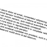
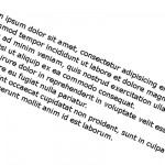
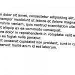
We will work on 5 different images of the same short (but famous) text.

The naming convention for those images is rather simple, the first letter stands for the sign of the angle (p for plus, m for minus) and the following number is the value of the angle.
m8.jpg has therefore been rotated by an angle of -8 degrees.

We assume here that the noise introduced by digitization has been removed by a previous preprocessing stage. We also assume that the text has been isolated: no images, horizontal or vertical separators, etc.

Implementation with OpenCV

First, let's declare a function compute_skew, it takes a path to an image as input and outputs the detected angle to standard output.
First we load the image and stores its size in a variable, very simple.

void compute_skew(const char* filename)
{
   // Load in grayscale.
   cv::Mat src = cv::imread(filename, 0);
   cv::Size size = src.size();

In image processing, objects are white and the background is black, we have the opposite, we need to invert the colors of our image:

   cv::bitwise_not(src, src);

And here is the result:

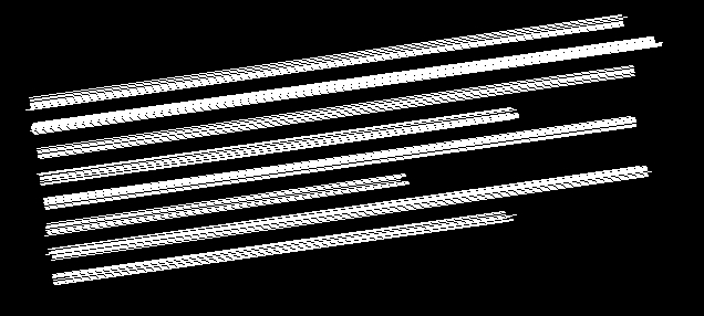
In order to compute the skew we must find straight lines in the text. In a text line, we have several letters side by side, lines should therefore be formed by finding long lines of white pixels in the image. Here is an example below:

Of course as characters have an height, we find several lines for each actual line from the text. By fine tuning the parameters used later or by using preprocessing we can decrease the number of lines.

So, how do we find lines in the image ? We use a powerful mathematical tool called the Hough transform. I won't dig into mathematical details, but the main idea of the Hough transform is to use a 2D accumulator in order to count how many times a given line has been found in the image, the whole image is scanned and by a voting system the "best" lines are identified.
We used a more efficient variant of the Standard Hough Transform (SHT) called the Probabilistic Hough Transform (PHT). In OpenCV the PHT is implemented under the name HoughLinesP.

In addition to the standard parameters of the Hough Transform, we have two additional parameters:

  • minLineLength – The minimum line length. Line segments shorter than that will be rejected. This is a great tool in order to prune out small residual lines.
  • maxLineGap – The maximum allowed gap between points on the same line to link them.
    This could be interesting for a multi-columns text, for example we could choose to not link lines from different text columns.

Back to C++ now, in OpenCV the PHT stores the end points of the line whereas the SHT stores the line in polar coordinates (relative to the origin). We need a vector in order to store all the end points:

    std::vector<cv::Vec4i> lines;

We are ready for the Hough transform now:

    cv::HoughLinesP(src, lines, 1, CV_PI/180, 100, size.width / 2.f, 20);

We use a step size of 1 for and for , the threshold (the minimum number of votes) is 100.
minLineLength is width/2, this is not an unreasonable assumption if the text is well isolated.
maxLineGap is 20, it seems a sound value for a gap.

In the remaining of the code we simply calculate the angle between each line and the horizontal line using the atan2 math function and we compute the mean angle of all the lines.
For debugging purposes we also draw all the lines in a new image called disp_lines and we display this image in a new window.

    cv::Mat disp_lines(size, CV_8UC1, cv::Scalar(0, 0, 0));
    double angle = 0.;
    unsigned nb_lines = lines.size();
    for (unsigned i = 0; i < nb_lines; ++i)
    {
        cv::line(disp_lines, cv::Point(lines[i][0], lines[i][1]),
                 cv::Point(lines[i][2], lines[i][3]), cv::Scalar(255, 0 ,0));
        angle += atan2((double)lines[i][3] - lines[i][1],
                       (double)lines[i][2] - lines[i][0]);
    }
    angle /= nb_lines; // mean angle, in radians.
 
    std::cout << "File " << filename << ": " << angle * 180 / CV_PI << std::endl;
 
    cv::imshow(filename, disp_lines);
    cv::waitKey(0);
    cv::destroyWindow(filename);
}

We just need a main function in order to call compute_skew on several images:

const char* files[] = { "m8.jpg", "m20.jpg", "p3.jpg", "p16.jpg", "p24.jpg"};
 
int main()
{
	unsigned nb_files = sizeof(files) / sizeof(const char*);
	for (unsigned i = 0; i < nb_files; ++i)
		compute_skew(files[i]);
}

That's all, here are the skew angles we obtain for each image, we have a pretty good accuracy: