Monthly Archives: September 2011

C++ - Getting started with SSE

In this article I will present how to use SSE instructions in C++ (or C).
My goal is not to show how to write the fastest possible program using SSE but rather to introduce to its usage.

What is SSE ?

SSE stands for Streaming SIMD Extensions. It is a set of CPU instructions dedicated to applications like signal processing, scientific computation or 3D graphics.

SIMD is an acronym itself: Single Instruction, Multiple Data. A CPU instruction is said to be SIMD when the same operation is applied on multiple data at the same time.

SSE was first introduced in the Pentium III in 1999. Over the time, this instruction set was improved by adding more sophisticated operations. Eight 128-bits registers were added to the CPU: xmm0 through xmm7.
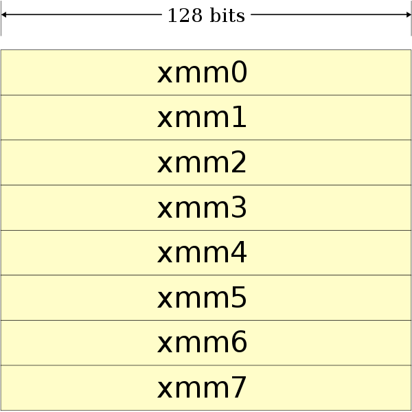
Initially those registers could only be used for single-precision computations (i.e. for the type float). But since SSE2, those registers can be used for any primitive data type.
Given a standard 32-bit machine we can therefore store and process in parallel:
- 2 double
- 2 long
- 4 float
- 4 int
- 8 short
- 16 char
Note that integer types can be signed or unsigned, but you will have to use (sometimes) different instructions.

For instance if you have to compute the sum of two int arrays, using SSE you can compute 4 additions in a single assembly instruction.

Simple program

It is not easy getting started with SSE, fortunately the MSDN documentation is complete and well-written.
If you take a look at the list of arithmetic operations you can notice there is always a corresponding assembly instruction. Some operations on the other side (such as set operations) are composite operations.
Using SSE in C++ is indeed a very low-level construct: we will manipulate directly the 128-bits registers through variables of type __m128 for float, __m128d for double and __m128i for int, short, char.

But the good news is that you don't need to declare arrays of type __m128 in order to use SSE: for instance if you want to calculate the square root of a large array of float, you can simply cast your pointer to the type __m128* and then use SSE operations.

There is a tweak however, most SSE operations requires the data to be 16-bytes aligned, here we will use another variable attributes of gcc.
We use the align attribute:

aligned (alignment)
This attribute specifies a minimum alignment for the variable or structure field, measured in bytes.

Here is a simple code on how to use SSE in order to compute the square root of 4 float in a single operation using the _mm_sqrt_ps function.

  float a[] __attribute__ ((aligned (16))) = { 41982.,  81.5091, 3.14, 42.666 };                                                                                                                                 
  __m128* ptr = (__m128*)a;                                                                                                                                                                                      
  __m128 t = _mm_sqrt_ps(*ptr);

The corresponding assembly instruction is SQRTPS, if we generate the assembly code of our program (using gcc -S) we can notice that this instruction is indeed used on a SSE register:

sqrtps  %xmm0, %xmm0

Don't forget the include !

  #include <emmintrin.h>

First benchmark

In the previous program we computed the square root of 4 float simultaneously but the result was not stored in the array. For this purpose we use _mm_store_ps.
In the following program we compute the square root of a very large array on float. We use the timer class presented here in order to measure the execution time of the SSE version against the standard version.

void normal(float* a, int N)                                                                                                                                                                                     
{                                                                                                                                                                                                                
  for (int i = 0; i < N; ++i)                                                                                                                                                                                    
    a[i] = sqrt(a[i]);                                                                                                                                                                                           
}                                                                                                                                                                                                                
 
void sse(float* a, int N)                                                                                                                                                                                        
{                      
  // We assume N % 4 == 0.                                                                                                                                                                                        
  int nb_iters = N / 4;                                                                                                                                                                                         
  __m128* ptr = (__m128*)a;                                                                                                                                                                                      
 
  for (int i = 0; i < nb_iters; ++i, ++ptr, a += 4)                                                                                                                                                              
    _mm_store_ps(a, _mm_sqrt_ps(*ptr));                                                                                                                                                                          
}                                                                                                                                                                                                                
 
int main(int argc, char** argv)                                                                                                                                                                                  
{                                                                                                                                                                                                                
  if (argc != 2)                                                                                                                                                                                                 
    return 1;                                                                                                                                                                                                    
  int N = atoi(argv[1]);                                                                                                                                                                                         
 
  float* a;                                                                                                                                                                                                      
  posix_memalign((void**)&a, 16,  N * sizeof(float));                                                                                                                                                            
 
  for (int i = 0; i < N; ++i)                                                                                                                                                                                    
    a[i] = 3141592.65358;                                                                                                                                                                                        
 
  {                                                                                                                                                                                                              
    TIMER("normal");                                                                                                                                                                                             
    normal(a, N);                                                                                                                                                                                                
  }                                                                                                                                                                                                              
 
  for (int i = 0; i < N; ++i)                                                                                                                                                                                    
    a[i] = 3141592.65358;                                                                                                                                                                                        
 
  {                                                                                                                                                                                                              
    TIMER("SSE");                                                                                                                                                                                                
    sse(a, N);                                                                                                                                                                                                   
  }
}

In the SSE function we use two pointers containing the same address but of different types, it is of course not necessary but avoid casting. It is also interesting to notice that we must increment the __m128 pointer by only 1 (128 bits) whereas we must increment the float pointer by 4 (32 bits).

Another interesting function here is the posix_memalign function instead of the align attribute. The first function allocates aligned data on the heap whereas the gcc attribute allocates on the stack.

The benchmark was compiled with llvm-g++ 4.2 (flags: -O3 -msse2) and ran on a Intel Core2 Duo P7350 (2GHz):

$ ./sqrt 64000000
normal: 392ms
SSE: 145ms

Pretty fast indeed !

Second Benchmark

And now how to add two arrays of char together:

void sse(char* a, const char* b, int N)                                                                                                                                                                          
{                                                                                                                                                                                                                
  int nb_iters = N / 16;                                                                                                                                                                                         
 
  __m128i* l = (__m128i*)a;                                                                                                                                                                                      
  __m128i* r = (__m128i*)b;                                                                                                                                                                                      
 
  for (int i = 0; i < nb_iters; ++i, ++l, ++r)                                                                                                                                                                   
    _mm_store_si128(l, _mm_add_epi8(*l, *r));                                                                                                                                                                    
}

And the benchmark with full optimizations turned on:

$ ./add 64000000
normal: 98ms
SSE: 42ms

Performance considerations

You may ask why we don't have a 4-fold speedup when we compute the square root of 4 float in a single instruction and why we only have a 2-fold speedup when we add 16 char at the same time.

The answer is that your compiler is smart and performs a lot of optimizations, especially at the O3 level. In fact, if you take a look at the generated assembly code for the "normal" version of the sort and add functions you will probably notice that your compiler used SSE instructions behind your back. The compiler detected a loop pattern suitable for SSE and therefore decided to use dedicated instructions, however using directly the SSE instructions the generated code was even faster.

Depending on your compiler version, for such simple loops it is possible that you will notice no difference in execution time, but as mentioned, my goal was not pure performances.


C++ - Resource Acquisition Is Initialization

Resource Acquisition Is Initialization

In the previous article we presented a simple timer class that initializes its internal clock in the constructor and computes the elapsed time in the destructor.

In fact, initializing a resource in a constructor and discarding it in a destructor is a common idiom in C++ called Resource Acquisition Is Initialization (RAII).
This is a great technique when dealing with exception handling: for example let's say at the beginning of a function you allocate 10 blocks of memory, open 2 files and acquire a lock. Of course you are really tidy so you properly free the allocated memory, close the files and release the lock at the end of the function.

However if an exception is raised in the middle of your code, you are in deep trouble: your program leaks memory, file descriptors are still opened and the lock is not released...
When leaving a block (even when an exception is raised), all variables allocated on the stack (i.e. local variables) are destroyed, this process is called stack unwinding.

Even if you are not concerned with exceptions, by using the RAII idiom you can write simpler code and there is no risk you accidentally forget to release a lock !
For example, using RAII with a lock:

// Before critical section
{ // Critical section !
  Lock lock(mutex); // Construct Lock object and acquire mutex.
  // Do some super critical stuff
  ...
  // End of scope: variable lock is destroyed and the mutex is released automatically.
}
// After critical section

auto_ptr

You can also use RAII to handle files or you can use it with raw pointers using the C++ std::auto_ptr class. When the variable reaches end of scope, the destructor automatically calls delete on the pointer. Using operator * we can manipulate an auto_ptr just like a pointer of the underlying type:

{                                                                                                                                                                                                                
  std::auto_ptr<int> p(new int);                                                                                                                                                                                 
  *p = 42;                                                                                                                                                                                                       
  std::cout << *p << std::endl;
  // Allocated memory is released.                                                                                                                                                                             
}

RAII in C

Using gcc variable attributes you can use the RAII idiom in C!
We use the cleanup attribute:

cleanup (cleanup_function)
The cleanup attribute runs a function when the variable goes out of scope. This attribute can only be applied to auto function scope variables; it may not be applied to parameters or variables with static storage duration. The function must take one parameter, a pointer to a type compatible with the variable. The return value of the function (if any) is ignored.

Wikipedia presents an example on how to automatically call fclose() on a file descriptor using the cleanup attribute:

#define RAII_VARIABLE(vartype,varname,initval,dtor) \
    void _dtor_ ## varname (vartype * v) { dtor(*v); } \
    vartype varname __attribute__((cleanup(_dtor_ ## varname))) = (initval)
 
void example_usage() {
  RAII_VARIABLE(FILE*, logfile, fopen("logfile.txt", "w+"), fclose);
  fputs("hello logfile!", logfile);
}

C++ - Timer Class

Timer Class

In C++ we often need to measure execution time of a small block or function call.
There are several ways to do this in C++, and it is a real pain to come up with both a portable and accurate version.
Using standard C++ only we can write a simple timer class in a few lines only using std::clock(). This function returns the number of clock ticks elapsed since the program was launched. Unfortunately, on some systems the precision of this function is terrible.

class Timer
{
public:
  Timer(const std::string& name)
    : name_ (name),
      start_ (std::clock())
    {
    }
  ~Timer()
    {
      double elapsed = (double(std::clock() - start_) / double(CLOCKS_PER_SEC));
      std::cout << name_ << ": " << int(elapsed * 1000) << "ms" << std::endl;
    }
private:
  std::string name_;
  std::clock_t start_;
};                                                                                                                                                                                                               
 
#define TIMER(name) Timer timer__(name);

An instance of the Timer class is created by providing a name. The constructor initializes the timer by using std::clock(). When the object is destroyed we compute the elapsed time and print it on standard output. We also define a macro TIMER(name) for convenience.

Usage

As the timer is initialized in the constructor and terminated in the destructor, we need to isolate the part of the code we want to measure in a block. When the end of the block is reached, we exit the scope of the timer variable and the destructor is called.
For example:

  int i = ...;
  for (...)
    ...
 
  {
    TIMER("Huge Loop"); // initialize timer
    for (...)
      ...
    // timer variable is destroyed: print elapsed time.
  }

The output can be something like this: Huge Loop: 352ms

User time VS Wall time

Good to know: by using std::clock() (instead of date-based methods) we measure user time, that is to say time actually spent by the CPU for the execution of the current program. If the process is put to sleep for a long time, we won't notice any change. For example the following code:

{
  TIMER("sleep");
  sleep(2); // go to sleep for 2s
}

should print this: sleep: 0ms.
If wall clock time was measured we would have approximately 2000ms here.

OpenCV - Morphological Skeleton

Skeleton

In many computer vision applications we often have to deal with huge amounts of data: processing can therefore be slow and requires a lot of memory.
In order to achieve faster processing and a smaller memory footprint, we sometimes use a more compact representation called a skeleton.
A skeleton must preserve the structure of the shape but all redundant pixels should be removed.
Here is a skeleton of the letter "B":

In this article we will present how to compute a morphological skeleton with the library OpenCV.
The skeleton obtained is far from perfect but it is a really simple method compared to other existing algorithms.

Pseudocode

As described on Wikipedia, a morphological skeleton can be computed using only the two basic morphological operations: dilate and erode.
In pseudo code, the algorithm works as follow:

img = ...;
while (not_empty(img))
{
    skel = skel | (img & !open(img));
    img = erosion(img);
}

At each iteration the image is eroded again and the skeleton is refined by computing the union of the current erosion less the opening of this erosion. An opening is simply an erosion followed by a dilation.

Implementation

It's really straightforward, first load the image to process in grayscale and transform it to a binary image using thresholding:

cv::Mat img = cv::imread("O.png", 0);
cv::threshold(img, img, 127, 255, cv::THRESH_BINARY);

We now need an image to store the skeleton and also a temporary image in order to store intermediate computations in the loop. The skeleton image is filled with black at the beginning.

cv::Mat skel(img.size(), CV_8UC1, cv::Scalar(0));
cv::Mat temp(img.size(), CV_8UC1);

We have to declare the structuring element we will use for our morphological operations, here we use a 3x3 cross-shaped structure element (i.e. we use 4-connexity).

cv::Mat element = cv::getStructuringElement(cv::MORPH_CROSS, cv::Size(3, 3));

And now the core of the algorithm, the main loop. We need a boolean variable in order to check if there is at least one pixel remaining. Operations are done in-place when possible.

bool done;
do
{
  cv::morphologyEx(img, temp, cv::MORPH_OPEN, element);
  cv::bitwise_not(temp, temp);
  cv::bitwise_and(img, temp, temp);
  cv::bitwise_or(skel, temp, skel);
  cv::erode(img, img, element);
 
  double max;
  cv::minMaxLoc(img, 0, &max);
  done = (max == 0);
} while (!done);

The use of the minMaxLoc function deserves an explanation. We want to check if there is still at least one pixel in the image, unfortunately I have not found a function for this task in OpenCV, therefore I just check if the maximum value is 0. minMaxLoc stores the minimum value in the second parameter (ignored if NULL pointer) and the maximum in the third parameter. A short-circuit OR function would be nice for this task.

The loop is over, we have our skeleton, let's display it!

cv::imshow("Skeleton", skel);
cv::waitKey(0);

Results

On a big "O":

On the word "OpenCV":

Optimization

As discussed with Arthur Kalverboer in the comments below, it is possible to optimize the computation in several ways.

First of all we can notice we perform the open operation and just after we perform an erosion on the same image, but an opening is just an erosion followed by a dilation, so we can perform the erosion and save it to a new image eroded, and at the end of the loop we copy eroded to img.

The second optimization concerns the use of cv::minMaxLoc in order to check if an image still has white pixels, computing the norm (cv::norm) of the image is faster.
EDIT2: Abid Rahman told me the function 'cv::countNonZero' is even faster, I didn't know this function existed, thanks!

Finally the last optimization is to replace the and and not operations by a simple set difference operation (cv::subtract). This works because we only manipulate binary images.

Here is the updated code:

cv::threshold(img, img, 127, 255, cv::THRESH_BINARY); 
cv::Mat skel(img.size(), CV_8UC1, cv::Scalar(0));
cv::Mat temp;
cv::Mat eroded;
 
cv::Mat element = cv::getStructuringElement(cv::MORPH_CROSS, cv::Size(3, 3));
 
bool done;		
do
{
  cv::erode(img, eroded, element);
  cv::dilate(eroded, temp, element); // temp = open(img)
  cv::subtract(img, temp, temp);
  cv::bitwise_or(skel, temp, skel);
  eroded.copyTo(img);
 
  done = (cv::countNonZero(img) == 0);
} while (!done);

Also, don't forget to crop your images before processing. The two images I gave as examples are not cropped, cropping them (manually or using OpenCV) also improves execution time.

OpenCV - Detect skew angle

OpenCV

Lately I have been interested in the library OpenCV. This library, initially developed by Intel, is dedicated to computer vision applications and is known to be one of the fastest (and maybe the fastest ?) library available for real-time computer vision.

And yet, if you think the library is not fast enough you can install Intel Integrated Performance Primitives (IPP) on your system and benefit from heavily optimized routines. If you have several cores available on your computer, you can also install Intel Threading Building Blocks (TBB). And if it's still not fast enough, you can run some operations on your GPU using CUDA !

All these features looked really exciting, so I decided to experiment a little bit with OpenCV in order to test its interface and expressive power. In this article I present a simple and very short project that detects the skew angle of a digitized document. My goal is not to present an error-proof program but rather to show the ease of use of OpenCV.

Skew angle

The detection of the skew angle of a document is a common preprocessing step in document analysis.

The document might have been slightly rotated during its digitization. It is therefore necessary to compute the skew angle and to rotate the text before going further in the processing pipeline (i.e. words/letters segmentation and later OCR).

We will work on 5 different images of the same short (but famous) text.

The naming convention for those images is rather simple, the first letter stands for the sign of the angle (p for plus, m for minus) and the following number is the value of the angle.
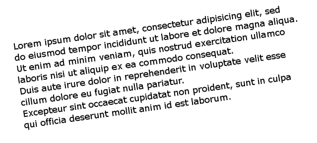
m8.jpg has therefore been rotated by an angle of -8 degrees.

We assume here that the noise introduced by digitization has been removed by a previous preprocessing stage. We also assume that the text has been isolated: no images, horizontal or vertical separators, etc.

Implementation with OpenCV

First, let's declare a function compute_skew, it takes a path to an image as input and outputs the detected angle to standard output.
First we load the image and stores its size in a variable, very simple.

void compute_skew(const char* filename)
{
   // Load in grayscale.
   cv::Mat src = cv::imread(filename, 0);
   cv::Size size = src.size();

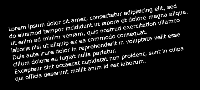
In image processing, objects are white and the background is black, we have the opposite, we need to invert the colors of our image:

   cv::bitwise_not(src, src);

And here is the result:

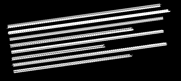
In order to compute the skew we must find straight lines in the text. In a text line, we have several letters side by side, lines should therefore be formed by finding long lines of white pixels in the image. Here is an example below:

Of course as characters have an height, we find several lines for each actual line from the text. By fine tuning the parameters used later or by using preprocessing we can decrease the number of lines.

So, how do we find lines in the image ? We use a powerful mathematical tool called the Hough transform. I won't dig into mathematical details, but the main idea of the Hough transform is to use a 2D accumulator in order to count how many times a given line has been found in the image, the whole image is scanned and by a voting system the "best" lines are identified.
We used a more efficient variant of the Standard Hough Transform (SHT) called the Probabilistic Hough Transform (PHT). In OpenCV the PHT is implemented under the name HoughLinesP.

In addition to the standard parameters of the Hough Transform, we have two additional parameters:

  • minLineLength – The minimum line length. Line segments shorter than that will be rejected. This is a great tool in order to prune out small residual lines.
  • maxLineGap – The maximum allowed gap between points on the same line to link them.
    This could be interesting for a multi-columns text, for example we could choose to not link lines from different text columns.

Back to C++ now, in OpenCV the PHT stores the end points of the line whereas the SHT stores the line in polar coordinates (relative to the origin). We need a vector in order to store all the end points:

    std::vector<cv::Vec4i> lines;

We are ready for the Hough transform now:

    cv::HoughLinesP(src, lines, 1, CV_PI/180, 100, size.width / 2.f, 20);

We use a step size of 1 for and for , the threshold (the minimum number of votes) is 100.
minLineLength is width/2, this is not an unreasonable assumption if the text is well isolated.
maxLineGap is 20, it seems a sound value for a gap.

In the remaining of the code we simply calculate the angle between each line and the horizontal line using the atan2 math function and we compute the mean angle of all the lines.
For debugging purposes we also draw all the lines in a new image called disp_lines and we display this image in a new window.

    cv::Mat disp_lines(size, CV_8UC1, cv::Scalar(0, 0, 0));
    double angle = 0.;
    unsigned nb_lines = lines.size();
    for (unsigned i = 0; i < nb_lines; ++i)
    {
        cv::line(disp_lines, cv::Point(lines[i][0], lines[i][1]),
                 cv::Point(lines[i][2], lines[i][3]), cv::Scalar(255, 0 ,0));
        angle += atan2((double)lines[i][3] - lines[i][1],
                       (double)lines[i][2] - lines[i][0]);
    }
    angle /= nb_lines; // mean angle, in radians.
 
    std::cout << "File " << filename << ": " << angle * 180 / CV_PI << std::endl;
 
    cv::imshow(filename, disp_lines);
    cv::waitKey(0);
    cv::destroyWindow(filename);
}

We just need a main function in order to call compute_skew on several images:

const char* files[] = { "m8.jpg", "m20.jpg", "p3.jpg", "p16.jpg", "p24.jpg"};
 
int main()
{
	unsigned nb_files = sizeof(files) / sizeof(const char*);
	for (unsigned i = 0; i < nb_files; ++i)
		compute_skew(files[i]);
}

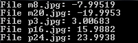
That's all, here are the skew angles we obtain for each image, we have a pretty good accuracy:

4D Julia Set

The project

During the last school year we had numerous maths courses: theory of distributions, model theory, Lie algebra... For this last course, we were given several projects idea by our teacher, we have chosen to make a 3D representation of the special linear group and of the Julia set.
An online representation of the Julia set can be found here.
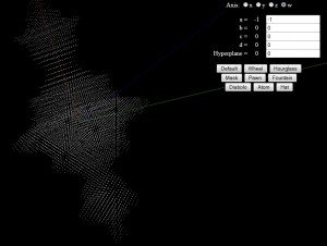
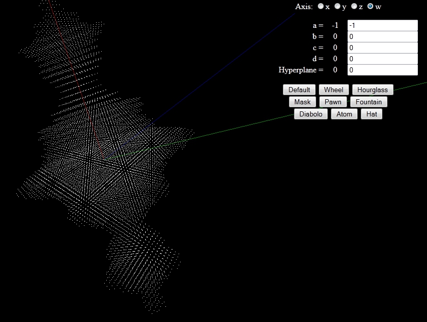
You can try some presetted values that yielded nice figures or you can mess around with the different parameters (explained in the following section).

Warning:
I recommend using a top notch web browser, if everything is black or you have only a 3D axis, try again with another browser.

This project was my first experiment with Javascript and WebGL using ThreeJS
Using JS was not a requirement for the project, but we thought it would be a good idea to have an online demo !

Explanations

Julia sets are fractals defined by the recurrence relation , with being a constant.
If, for a given , converges, then is in the Julia set.

Julia sets can be represented in 2D (as shown on wikipedia) with ) or in 4D with .
is the set of quaternions, quaternions are hypercomplex numbers of the following form:


With , , being roots of unity, i.e. .

To obtain a representation in a 4D space, each point of this space is represented by a quaternion.
Given a fixed value of , we can compute the corresponding Julia set by testing the convergence of for all points of this 4D space.
In our online demo, the 4 coefficients of the quaternion constant can be modified through the sliders , , and .

We cannot visualize 4D objects, so we need a 3D representation of the Julia set. We have to take a slice of the Julia set, in other words we compute the intersection of the set with an hyperplane.
What this means for our demo is that we assign a constant value to the same coefficient for each quaternion (for example the coefficient associated with ).
The three remaining coefficients will form the three axis of our 3D representation (, et ).
In our online demo we can choose which coefficient should be fixed and modify its value with the slider Hyperplane.

Once we have fixed a coefficient for all quaternions, we iterate through all possible values of , and .
For instance if we have chosen that , the initial value of the sequence is therefore:

Point is in the Julia set (and hence displayed as a white dot) if, after a given number of iterations, the sequence is below a threshold. In our demo we compute 10 iterations.